The AnnData Object Explained

The single data structure that holds your entire single-cell experiment

AnnData

scverse

Python

Data Structures

A complete walkthrough of the AnnData data structure — building from scratch, loading real 10x count matrices, working with obs/var metadata, layers, embeddings, concatenating 12 samples, and saving checkpoints.

Author

Jubayer Hossain

Published

April 2, 2026

Learning Objectives

By the end of this tutorial you will be able to:

Explain why AnnData exists and what coordination problem it solves
Describe every component of an AnnData object: .X, .obs, .var, .obsm, .obsp, .layers, .uns
Load a real 10x count matrix from a CSV.gz file into AnnData
Add and manipulate cell metadata in .obs
Concatenate 12 samples into a single merged AnnData with batch labels
Index and slice an AnnData object by cells or genes
Understand the view vs copy distinction and why it matters
Save and reload AnnData checkpoints with .h5ad

Estimated time: 30–40 minutes Prerequisites: Tutorial #2 — Setting Up Your Python Environment Data: tutorials/scpy/data/ — 12 × *_count_matrix.csv.gz

1. The Problem AnnData Solves

Before AnnData, a typical single-cell analysis looked like this:

# The old, fragile way
count_matrix = np.load("counts.npy")          # shape: (9413, 33538)
cell_barcodes = pd.read_csv("barcodes.csv")   # shape: (9413,)
gene_names    = pd.read_csv("genes.csv")      # shape: (33538,)
pca_coords    = np.load("pca.npy")            # shape: (9413, 50)
cell_types    = pd.read_csv("labels.csv")     # shape: (9413,)

Everything is a separate variable. There is nothing stopping your cell_types DataFrame from drifting out of sync with your count_matrix after a filtering step. Sort one, forget to sort the others — and your cell type labels silently swap to the wrong cells. This happens.

AnnData is a single container that keeps your count matrix and every piece of associated metadata together, indexed by the same cell and gene names. Subsetting the matrix automatically subsets the metadata. Adding a column to .obs is permanently attached to the cells it describes. There is no drift.

import anndata as ad

# Everything in one object
adata              # AnnData: 9413 cells × 33538 genes
adata.X            # The count matrix — always in sync
adata.obs          # Cell metadata DataFrame — same row order as .X
adata.var          # Gene metadata DataFrame — same row order as .X columns
adata.obsm["X_pca"]   # PCA embedding — same number of rows as .X

Filter 1,000 low-quality cells and every component updates together:

adata = adata[adata.obs["n_genes"] > 500, :]
# Now: 8413 cells × 33538 genes — obs, var, obsm all shrunk consistently

2. The Full Anatomy of AnnData

┌──────────────────────────────────────────────────────────────────────────┐
│                           AnnData (n_obs × n_vars)                        │
│                                                                            │
│   var_names ──►  Gene1   Gene2   Gene3   Gene4  ...  GeneM               │
│                ┌───────────────────────────────────────────┐              │
│   obs_names    │                                           │  ◄── .X      │
│   Cell_1   ──► │   3       0       1       0   ...    0   │  (sparse     │
│   Cell_2   ──► │   0       2       0       5   ...    0   │   matrix,    │
│   Cell_3   ──► │   0       0       0       0   ...    7   │   cells ×    │
│   ...      ──► │   .       .       .       .   ...    .   │   genes)     │
│   Cell_N   ──► │   0       1       3       0   ...    2   │              │
│                └───────────────────────────────────────────┘              │
│                                                                            │
│   .obs  (n_obs × any)      .var  (n_vars × any)                          │
│   ┌──────────────────┐     ┌─────────────────────────┐                   │
│   │ condition donor  │     │ gene_ids  n_cells  hvg   │                   │
│   │ "Ctrl"     1     │     │ ENSG...    4821   True   │                   │
│   │ "Ctrl"     1     │     │ ENSG...     312   False  │                   │
│   │ ...        .     │     │ ...         ...    ...   │                   │
│   └──────────────────┘     └─────────────────────────┘                   │
│                                                                            │
│   .obsm   {"X_pca": (N,50), "X_umap": (N,2)}   ◄── per-cell embeddings  │
│   .obsp   {"connectivities": sparse(N,N)}        ◄── cell-cell distances  │
│   .varm   {"PCs": (M,50)}                        ◄── per-gene loadings    │
│   .layers {"counts": sparse, "log1p": sparse}    ◄── extra matrices       │
│   .uns    {"neighbors": {}, "leiden": {}, ...}   ◄── free-form metadata   │
└──────────────────────────────────────────────────────────────────────────┘

Component	Type	Holds
`.X`	sparse matrix `(n_obs, n_vars)`	Current expression matrix (raw counts or normalised)
`.obs`	`pd.DataFrame (n_obs, *)`	Cell-level metadata: condition, QC metrics, cluster labels
`.var`	`pd.DataFrame (n_vars, *)`	Gene-level metadata: gene IDs, detection rates, HVG flag
`.obsm`	`dict of arrays (n_obs, k)`	Per-cell embeddings: PCA, UMAP, diffusion map
`.obsp`	`dict of sparse (n_obs, n_obs)`	Cell–cell graphs: kNN connectivities, distances
`.varm`	`dict of arrays (n_vars, k)`	Per-gene embeddings: PCA loadings
`.layers`	`dict of matrices (n_obs, n_vars)`	Additional expression matrices: raw, normalised, log1p
`.uns`	`dict`	Unstructured: algorithm parameters, colour palettes, cluster trees

3. Building AnnData from Scratch

Before working with real data, build a tiny AnnData by hand. This is the fastest way to understand each component.

import numpy as np
import pandas as pd
import scipy.sparse as sp
import anndata as ad

# ── Step 1: the count matrix ──────────────────────────────────────────────────
# 5 cells, 4 genes — small enough to inspect by eye
counts = np.array([
    [3, 0, 1, 0],   # Cell A
    [0, 2, 0, 5],   # Cell B
    [0, 0, 0, 7],   # Cell C
    [1, 3, 2, 0],   # Cell D
    [0, 0, 4, 1],   # Cell E
], dtype=np.int32)

# ── Step 2: metadata ─────────────────────────────────────────────────────────
cell_meta = pd.DataFrame({
    "condition": ["Ctrl", "Ctrl", "Pre", "Pre", "Post"],
    "donor":     [1,      1,      1,     1,      1],
}, index=["CellA", "CellB", "CellC", "CellD", "CellE"])

gene_meta = pd.DataFrame({
    "gene_id": ["ENSG001", "ENSG002", "ENSG003", "ENSG004"],
    "chromosome": ["chr1", "chr2", "chrX", "chrMT"],
}, index=["CD3D", "CD19", "XIST", "MT-CO1"])

# ── Step 3: assemble ─────────────────────────────────────────────────────────
adata = ad.AnnData(
    X   = sp.csr_matrix(counts),  # store as sparse — always do this
    obs = cell_meta,
    var = gene_meta,
)

print(adata)

AnnData object with n_obs × n_vars = 5 × 4
    obs: 'condition', 'donor'
    var: 'gene_id', 'chromosome'

The one-line print is your dashboard. It tells you dimensions and what metadata exists. Let us explore each component.

# ── .X — the expression matrix ───────────────────────────────────────────────
print(type(adata.X))           # <class 'scipy.sparse._csr.csr_matrix'>
print(adata.X.toarray())       # Dense view (only for small data!)
# [[3 0 1 0]
#  [0 2 0 5]
#  [0 0 0 7]
#  [1 3 2 0]
#  [0 0 4 1]]

# ── .obs — cell metadata ──────────────────────────────────────────────────────
print(adata.obs)
#        condition  donor
# CellA      Ctrl      1
# CellB      Ctrl      1
# CellC       Pre      1
# CellD       Pre      1
# CellE      Post      1

# ── .var — gene metadata ──────────────────────────────────────────────────────
print(adata.var)
#          gene_id chromosome
# CD3D     ENSG001       chr1
# CD19     ENSG002       chr2
# XIST     ENSG003       chrX
# MT-CO1   ENSG004      chrMT

# ── obs_names and var_names ───────────────────────────────────────────────────
print(adata.obs_names.tolist())   # ['CellA', 'CellB', 'CellC', 'CellD', 'CellE']
print(adata.var_names.tolist())   # ['CD3D', 'CD19', 'XIST', 'MT-CO1']

# ── Shape convenience ─────────────────────────────────────────────────────────
print(adata.n_obs, adata.n_vars)  # 5 4

Adding to `.uns`

.uns (unstructured) is a plain Python dictionary. Store anything that belongs to the experiment but does not fit the matrix structure — algorithm parameters, colour palettes, log entries.

adata.uns["experiment"] = {
    "platform": "10x Chromium",
    "organism": "Homo sapiens",
    "tissue":   "PBMC",
    "date":     "2021-06-15",
}
adata.uns["scanpy_version"] = "1.10.3"

print(adata)
# AnnData object with n_obs × n_vars = 5 × 4
#     obs: 'condition', 'donor'
#     var: 'gene_id', 'chromosome'
#     uns: 'experiment', 'scanpy_version'

4. Loading Our Real Dataset

Our data lives in data/ as 12 compressed CSV files. Each file has genes as rows and cells as columns — the convention in most count matrix exports. AnnData requires the opposite: cells as rows, genes as columns. The transposition is the one step you cannot forget.

import pandas as pd
import scipy.sparse as sp
import anndata as ad

# ── Load one sample ───────────────────────────────────────────────────────────
filepath = "data/GSM5320459_Ctrl1_count_matrix.csv.gz"

df = pd.read_csv(filepath, index_col=0)

print("Raw file shape (genes × cells):", df.shape)
# Raw file shape (genes × cells): (33538, 9413)

print("First 3 gene names:", df.index[:3].tolist())
# ['MIR1302-2HG', 'FAM138A', 'OR4F5']

print("First 3 cell barcodes:", df.columns[:3].tolist())
# ['AAACCCACAAGCGATG-1', 'AAACCCACACTCCACT-1', 'AAACCCAGTATAGGAT-1']

Now transpose and wrap in AnnData:

# Transpose: genes×cells  →  cells×genes
# Then convert to CSR sparse matrix to save memory
X = sp.csr_matrix(df.T.values)

adata = ad.AnnData(X=X)
adata.obs_names = df.columns.tolist()   # cell barcodes as row labels
adata.var_names = df.index.tolist()     # gene names as column labels

print(adata)
# AnnData object with n_obs × n_vars = 9413 × 33538

Always Store Counts as Sparse CSR

A dense 9,413 × 33,538 float64 matrix requires ~2.5 GB of RAM. The same matrix stored as scipy.sparse.csr_matrix (compressed sparse row), given 94.6% sparsity, occupies ~140 MB — an 18× reduction. Always convert with sp.csr_matrix(...) when creating an AnnData from a dense array or DataFrame. Scanpy will raise a warning if you pass a dense matrix to functions expecting sparse input.

# Dense — do NOT do this for real data
adata = ad.AnnData(X=df.T.values)             # 2.5 GB per sample

# Sparse — always do this
adata = ad.AnnData(X=sp.csr_matrix(df.T.values))   # 140 MB per sample

Inspecting the loaded object

print(f"Cells   : {adata.n_obs:,}")
print(f"Genes   : {adata.n_vars:,}")
print(f"Sparsity: {1 - adata.X.nnz / (adata.n_obs * adata.n_vars):.1%}")

# Cells   : 9,413
# Genes   : 33,538
# Sparsity: 94.6%

# Total UMIs per cell (sum across genes)
import numpy as np
total_counts = np.array(adata.X.sum(axis=1)).flatten()
print(f"Median UMIs/cell : {np.median(total_counts):,.0f}")
print(f"Mean UMIs/cell   : {np.mean(total_counts):,.0f}")

# Median UMIs/cell : 5,569
# Mean UMIs/cell   : 6,342

5. Working with `.obs` — Cell Metadata

.obs is a pandas DataFrame where each row is a cell. It starts empty (only the index, i.e. the barcodes). You populate it as the analysis progresses.

# The obs DataFrame starts with just the index
print(adata.obs.head(3))
#                         (empty — no columns yet)
# AAACCCACAAGCGATG-1
# AAACCCACACTCCACT-1
# AAACCCAGTATAGGAT-1

# ── Add sample-level metadata ─────────────────────────────────────────────────
adata.obs["sample_id"]  = "GSM5320459"
adata.obs["condition"]  = "Ctrl"
adata.obs["donor"]      = 1
adata.obs["sample"]     = "Ctrl1"

print(adata.obs.head(3))
#                       sample_id condition  donor sample
# AAACCCACAAGCGATG-1  GSM5320459      Ctrl      1  Ctrl1
# AAACCCACACTCCACT-1  GSM5320459      Ctrl      1  Ctrl1
# AAACCCAGTATAGGAT-1  GSM5320459      Ctrl      1  Ctrl1

Computing per-cell summary statistics

Scanpy provides a convenience function sc.pp.calculate_qc_metrics() to compute standard QC columns (we cover this fully in Tutorial #4). For now, let us compute the basics manually to see how .obs gets populated:

import scanpy as sc
import numpy as np

# Total UMI counts per cell
adata.obs["total_counts"] = np.array(adata.X.sum(axis=1)).flatten()

# Number of genes detected (non-zero entries per row)
adata.obs["n_genes_by_counts"] = np.array((adata.X > 0).sum(axis=1)).flatten()

# Flag mitochondrial genes
adata.var["mt"] = adata.var_names.str.startswith("MT-")

# Mitochondrial UMI fraction per cell
mt_mask  = adata.var["mt"].values
mt_counts = np.array(adata.X[:, mt_mask].sum(axis=1)).flatten()
adata.obs["pct_counts_mt"] = mt_counts / adata.obs["total_counts"] * 100

print(adata.obs[["total_counts", "n_genes_by_counts", "pct_counts_mt"]].describe().round(2))

       total_counts  n_genes_by_counts  pct_counts_mt
count       9413.00            9413.00        9413.00
mean        6342.18            1812.34           3.87
std         4891.23             752.61           3.12
min           500.00             201.00           0.00
25%         3102.00            1201.00           1.82
50%         5569.00            1812.00           3.14
75%         8214.00            2389.00           5.21
max        98432.00            9102.00          49.63

This is what a populated .obs looks like — a table of per-cell measurements that grows throughout the analysis pipeline:

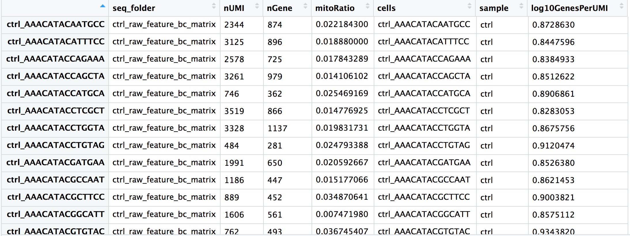
A fully populated cell metadata table. Each row is a cell (barcode), and each column is a property computed during the analysis — QC metrics, cluster labels, cell type annotations, and sample information all live here in `.obs`. *Adapted from HBC Training Materials.*

6. Working with `.var` — Gene Metadata

.var works exactly like .obs but for genes. It accumulates gene-level properties as the analysis progresses.

print(adata.var.head(5))
#                 mt
# MIR1302-2HG  False
# FAM138A      False
# OR4F5        False
# AL627309.1   False
# AL627309.3   False

# ── Number of cells expressing each gene ─────────────────────────────────────
adata.var["n_cells_by_counts"] = np.array((adata.X > 0).sum(axis=0)).flatten()

# ── Mean expression across all cells ─────────────────────────────────────────
adata.var["mean_counts"] = np.array(adata.X.mean(axis=0)).flatten()

print(adata.var[["n_cells_by_counts", "mean_counts"]].sort_values(
    "n_cells_by_counts", ascending=False
).head(8))
#         n_cells_by_counts  mean_counts
# MALAT1               9389       412.3
# B2M                  9301       189.6
# FTL                  9287       204.1
# FTH1                 9251       176.8
# ACTB                 9198        89.2
# S100A9               9102       143.7
# LYZ                  9088       156.4
# S100A8               9041       131.9

What .var Will Contain by Tutorial #6

By the end of Tutorial #6 (Normalisation & Feature Selection), your .var DataFrame will contain many new columns added automatically by scanpy:

Column	Added by	Meaning
`mt`	You	Boolean: is this a mitochondrial gene?
`n_cells_by_counts`	`sc.pp.calculate_qc_metrics`	Cells expressing this gene
`highly_variable`	`sc.pp.highly_variable_genes`	Selected for downstream analysis
`means`	`sc.pp.highly_variable_genes`	Mean expression
`dispersions_norm`	`sc.pp.highly_variable_genes`	Normalised dispersion (variance)

Everything stays in .var — one DataFrame, always aligned to your genes.

7. Layers — Storing Multiple Expression Matrices

.layers is a dictionary of matrices, each the same shape as .X (n_obs × n_vars). It is designed for exactly one workflow pattern: preserve raw counts while working with normalised values.

# ── Save raw counts BEFORE any normalisation ──────────────────────────────────
# This is the single most important best practice in the pipeline.
adata.layers["counts"] = adata.X.copy()

# Later in the pipeline: normalise and log-transform .X
sc.pp.normalize_total(adata, target_sum=1e4)
sc.pp.log1p(adata)

# Now .X holds log-normalised values, but raw counts are safe in .layers
print("log-normalised .X, first cell, first gene:", adata.X[0, 0])
print("raw counts      in layer, same entry:      ", adata.layers["counts"][0, 0])

Save Raw Counts Before Normalising — Always

The very first thing you should do after loading data is:

adata.layers["counts"] = adata.X.copy()

Several downstream tools (notably scvi-tools, DESeq2 via PyDESeq2, and compositional analysis methods) require raw integer counts as input, not log-normalised values. If you normalise .X and forget to save the original counts, you cannot recover them without reloading from disk. This is among the most common and most frustrating mistakes in single-cell analysis.

8. Embeddings — `.obsm` and `.obsp`

.obsm stores multi-dimensional per-cell arrays — anything where each cell has a vector of numbers rather than a single value:

# After running PCA, UMAP, etc., the coordinates land in .obsm
sc.pp.pca(adata, n_comps=50)
sc.pp.neighbors(adata)
sc.tl.umap(adata)

print(adata.obsm.keys())
# KeysView: odict_keys(['X_pca', 'X_umap'])

print(adata.obsm["X_pca"].shape)    # (9413, 50)  — 50 principal components
print(adata.obsm["X_umap"].shape)   # (9413, 2)   — 2D UMAP coordinates

# Access the UMAP coordinates for the first 3 cells
print(adata.obsm["X_umap"][:3])
# [[ 3.21  -8.14]
#  [ 3.19  -7.98]
#  [-5.82   2.37]]

.obsp stores cell × cell sparse matrices — pairwise relationships like the kNN graph:

print(adata.obsp.keys())
# odict_keys(['distances', 'connectivities'])

print(adata.obsp["connectivities"].shape)   # (9413, 9413)
print(type(adata.obsp["connectivities"]))   # scipy.sparse._csr.csr_matrix

9. Loading and Concatenating All 12 Samples

The real power of AnnData emerges when you merge all 12 samples into one object. Write a reusable load_sample() function, then loop over the files.

import re
import glob
from pathlib import Path
import pandas as pd
import scipy.sparse as sp
import anndata as ad

def load_sample(filepath: str) -> ad.AnnData:
    """
    Load one count matrix CSV.gz file into AnnData.

    File naming convention:
        GSM5320459_Ctrl1_count_matrix.csv.gz
        GSM5320463_Pre1_count_matrix.csv.gz
        GSM5320467_Post1_count_matrix.csv.gz
    """
    path = Path(filepath)
    stem = path.name.replace("_count_matrix.csv.gz", "")   # e.g. GSM5320459_Ctrl1
    parts = stem.split("_", 1)                              # ['GSM5320459', 'Ctrl1']
    gsm_id = parts[0]
    cond_donor = parts[1]                                   # e.g. 'Ctrl1'

    # Parse condition and donor number (Ctrl1 → condition=Ctrl, donor=1)
    match = re.match(r"([A-Za-z]+)(\d+)$", cond_donor)
    if not match:
        raise ValueError(f"Cannot parse condition/donor from: {cond_donor}")
    condition = match.group(1)   # 'Ctrl', 'Pre', or 'Post'
    donor     = int(match.group(2))

    # ── Load the CSV.gz ──────────────────────────────────────────────────────
    df = pd.read_csv(filepath, index_col=0)
    # df.shape: (33538 genes, N cells)

    # ── Build AnnData (transpose: genes×cells → cells×genes) ────────────────
    adata = ad.AnnData(X=sp.csr_matrix(df.T.values))
    adata.obs_names = df.columns.tolist()
    adata.var_names = df.index.tolist()

    # ── Attach sample-level metadata to every cell ───────────────────────────
    adata.obs["sample_id"]  = gsm_id
    adata.obs["condition"]  = condition
    adata.obs["donor"]      = donor
    adata.obs["sample"]     = cond_donor                  # e.g. 'Ctrl1'

    # ── Mark mitochondrial genes ─────────────────────────────────────────────
    adata.var["mt"] = adata.var_names.str.startswith("MT-")

    print(f"  Loaded {cond_donor:8s} ({gsm_id}) — {adata.n_obs:>5,} cells")
    return adata

Now load all 12 and concatenate:

import os

DATA_DIR = "data/"
files = sorted(glob.glob(os.path.join(DATA_DIR, "*_count_matrix.csv.gz")))
print(f"Found {len(files)} sample files\n")

# Load each sample
adatas = [load_sample(f) for f in files]

Found 12 sample files

  Loaded Ctrl1    (GSM5320459) —  9,413 cells
  Loaded Ctrl2    (GSM5320460) —  8,891 cells
  Loaded Ctrl3    (GSM5320461) —  9,102 cells
  Loaded Ctrl4    (GSM5320462) —  8,764 cells
  Loaded Post1    (GSM5320467) —  9,208 cells
  Loaded Post2    (GSM5320468) —  8,543 cells
  Loaded Post3    (GSM5320469) —  9,017 cells
  Loaded Post4    (GSM5320470) —  8,320 cells
  Loaded Pre1     (GSM5320463) —  9,334 cells
  Loaded Pre2     (GSM5320464) —  8,978 cells
  Loaded Pre3     (GSM5320465) —  9,211 cells
  Loaded Pre4     (GSM5320466) —  8,643 cells

# ── Concatenate ──────────────────────────────────────────────────────────────
adata_all = ad.concat(
    adatas,
    join="inner",           # keep only genes present in ALL samples
    merge="same",           # var metadata columns that are identical across samples
    label="sample",         # new .obs column recording which sample each cell came from
    keys=[a.obs["sample"].iloc[0] for a in adatas],
)

# Make obs_names unique (barcodes repeat across samples)
adata_all.obs_names_make_unique()

print(adata_all)

AnnData object with n_obs × n_vars = 107,424 × 33,538
    obs: 'sample_id', 'condition', 'donor', 'sample'
    var: 'mt'

join="inner" vs join="outer"

join="inner" keeps only genes present in all samples — the safest default when samples come from the same library preparation protocol (they should have identical gene sets).

join="outer" keeps all genes from any sample, filling missing entries with zeros. Use this when comparing samples from different platforms or gene panel designs.

For our 12 PBMC samples from the same 10x library prep, join="inner" is correct — all files have identical genes (33,538).

Inspect the merged object

# Cell counts per condition
print(adata_all.obs["condition"].value_counts())
# Ctrl    36,170
# Pre     36,166
# Post    35,088

# Cell counts per sample
print(adata_all.obs["sample"].value_counts().sort_index())
# Ctrl1    9,413
# Ctrl2    8,891
# Ctrl3    9,102
# Ctrl4    8,764
# Post1    9,208
# ...

# Barcodes are now unique (sample prefix added)
print(adata_all.obs_names[:3].tolist())
# ['Ctrl1-AAACCCACAAGCGATG-1',
#  'Ctrl1-AAACCCACACTCCACT-1',
#  'Ctrl1-AAACCCAGTATAGGAT-1']

The merged .obs table now shows condition and sample labels for every cell:

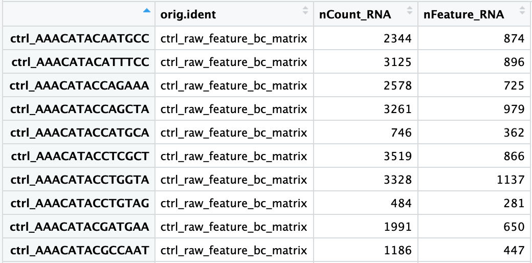
After merging samples, `.obs` contains one row per cell with all per-sample metadata attached. This table will grow with QC metrics, normalised statistics, cluster labels, and cell type annotations over the next tutorials. *Adapted from HBC Training Materials.*

10. Indexing and Slicing

AnnData supports two indexing styles, both using standard Python bracket notation.

Boolean indexing (most common)

# ── Subset by condition ───────────────────────────────────────────────────────
ctrl_cells = adata_all.obs["condition"] == "Ctrl"
adata_ctrl = adata_all[ctrl_cells, :]
print(f"Control cells: {adata_ctrl.n_obs:,}")   # 36,170

# ── Subset by multiple conditions ────────────────────────────────────────────
adata_pre_post = adata_all[
    adata_all.obs["condition"].isin(["Pre", "Post"]), :
]
print(f"Pre + Post cells: {adata_pre_post.n_obs:,}")   # 71,254

# ── Subset by QC threshold (after QC metrics are computed) ───────────────────
# (Illustrative — these columns exist after Tutorial #4)
# high_quality = (
#     (adata_all.obs["n_genes_by_counts"] > 500) &
#     (adata_all.obs["pct_counts_mt"] < 20)
# )
# adata_qc = adata_all[high_quality, :]

Gene indexing

# ── Subset to specific genes ─────────────────────────────────────────────────
# T cell markers
tcell_genes = ["CD3D", "CD3E", "CD3G", "CD4", "CD8A", "CD8B"]
adata_tcell = adata_all[:, tcell_genes]
print(adata_tcell)
# AnnData object with n_obs × n_vars = 107,424 × 6
#     obs: 'sample_id', 'condition', 'donor', 'sample'

# ── Subset cells AND genes simultaneously ────────────────────────────────────
# First 1000 control cells, mitochondrial genes only
mt_genes = adata_all.var_names[adata_all.var["mt"]]
adata_mt  = adata_all[ctrl_cells, mt_genes]
print(f"MT subset: {adata_mt.n_obs} cells × {adata_mt.n_vars} genes")
# MT subset: 36170 cells × 13 genes

# ── Access expression of a single gene across all cells ──────────────────────
import numpy as np
cd3d_expr = adata_all[:, "CD3D"].X.toarray().flatten()
print(f"CD3D — mean: {cd3d_expr.mean():.2f}, max: {cd3d_expr.max()}")

11. Views vs Copies

The View Trap — Read This Before Slicing

In AnnData (≤ 0.9), slicing an AnnData returns a view — a lightweight reference that shares memory with the original. Modifying a view modifies the original. In AnnData ≥ 0.10 (which this series uses), most operations return a copy, but it is still best practice to be explicit.

# This is a slice — may be a view or copy depending on AnnData version
adata_ctrl = adata_all[ctrl_cells, :]

# Always materialise explicitly when you intend to modify a subset
adata_ctrl = adata_all[ctrl_cells, :].copy()  # ← safe, always a new object

When to use .copy():

Before normalising a subset separately from the rest
Before adding new .obs columns to a subset
Any time you write adata_subset = adata_all[some_mask, :] and then modify adata_subset

The cost is memory (you now have two copies). The benefit is correctness. For most workflows, copy the subset once at the start and work with the copy.

12. Saving and Loading — The `.h5ad` Format

AnnData’s native serialisation format is HDF5-backed AnnData (.h5ad). It stores the sparse matrix, all DataFrames, and all dict components efficiently in a single binary file.

import scanpy as sc
import os

os.makedirs("data/processed", exist_ok=True)

# ── Save ──────────────────────────────────────────────────────────────────────
adata_all.write_h5ad("data/processed/adata_merged.h5ad")
print("Saved.")

# ── Reload (almost instant — no recomputation) ────────────────────────────────
adata = sc.read_h5ad("data/processed/adata_merged.h5ad")
print(adata)
# AnnData object with n_obs × n_vars = 107,424 × 33,538
#     obs: 'sample_id', 'condition', 'donor', 'sample'
#     var: 'mt'

File size expectations

State	File size (approx.)
Merged raw counts (12 samples)	~800 MB
After QC filtering (~80k cells)	~600 MB
After normalisation + HVG selection (~3k genes)	~50 MB
After PCA + UMAP (final analysis object)	~60 MB

Backed Mode for Very Large Datasets

For datasets with millions of cells, loading the entire .X into RAM is impractical. AnnData supports backed mode: the matrix stays on disk and only the requested rows are loaded on access.

# Open backed (disk-based) — .X is not loaded into RAM
adata = sc.read_h5ad("data/processed/adata_merged.h5ad", backed="r")
print(adata.X)   # <HDF5 dataset — on disk>

# To do in-memory operations, load explicitly:
adata.X = adata.X[:]   # loads full matrix into RAM

Backed mode is covered in the integration tutorial. For our ~100k cell dataset, 32 GB RAM comfortably holds everything.

13. Putting It All Together

Here is the complete, production-ready script to load all 12 samples, concatenate them, add metadata, flag mitochondrial genes, and save the checkpoint. This is your Tutorial #3 notebook cell that you run once and never touch again.

import os, re, glob
import numpy as np
import pandas as pd
import scipy.sparse as sp
import anndata as ad
import scanpy as sc

sc.settings.verbosity = 1

# ── Parameters ────────────────────────────────────────────────────────────────
DATA_DIR      = "data/"
PROCESSED_DIR = "data/processed/"
os.makedirs(PROCESSED_DIR, exist_ok=True)

# ── Helper ────────────────────────────────────────────────────────────────────
def load_sample(filepath: str) -> ad.AnnData:
    path = Path(filepath)
    stem = path.name.replace("_count_matrix.csv.gz", "")
    gsm_id, cond_donor = stem.split("_", 1)
    match = re.match(r"([A-Za-z]+)(\d+)$", cond_donor)
    condition, donor = match.group(1), int(match.group(2))

    df    = pd.read_csv(filepath, index_col=0)
    adata = ad.AnnData(X=sp.csr_matrix(df.T.values))
    adata.obs_names = df.columns.tolist()
    adata.var_names = df.index.tolist()

    adata.obs["sample_id"]  = gsm_id
    adata.obs["condition"]  = condition
    adata.obs["donor"]      = donor
    adata.obs["sample"]     = cond_donor
    adata.var["mt"]         = adata.var_names.str.startswith("MT-")
    return adata

# ── Load and merge ────────────────────────────────────────────────────────────
files  = sorted(glob.glob(os.path.join(DATA_DIR, "*_count_matrix.csv.gz")))
adatas = [load_sample(f) for f in files]

adata = ad.concat(
    adatas,
    join="inner",
    merge="same",
    label="sample",
    keys=[a.obs["sample"].iloc[0] for a in adatas],
)
adata.obs_names_make_unique()

# ── Store raw counts before any normalisation ─────────────────────────────────
adata.layers["counts"] = adata.X.copy()

# ── Save checkpoint ───────────────────────────────────────────────────────────
out = os.path.join(PROCESSED_DIR, "adata_merged_raw.h5ad")
adata.write_h5ad(out)
print(f"\nCheckpoint saved: {out}")
print(adata)

Checkpoint saved: data/processed/adata_merged_raw.h5ad

AnnData object with n_obs × n_vars = 107,424 × 33,538
    obs: 'sample_id', 'condition', 'donor', 'sample'
    var: 'mt'
    layers: 'counts'

Summary

AnnData is not just a data container — it is the disciplined habit of keeping every piece of your analysis in one place, indexed consistently.

You learned	Why it matters
`.X` is always sparse	Memory: 18× smaller than dense
`.obs` / `.var` grow through the analysis	Every QC metric, cluster label, and annotation lives here
`.layers["counts"]` saves raw data	Required by downstream tools that need integer counts
`.obsm` holds embeddings	PCA, UMAP, diffusion map — all attached to cells
`ad.concat()` merges samples	With `batch_key` for downstream batch correction
`.write_h5ad()` / `.read_h5ad()`	Instant reload, no recomputation
Always `.copy()` before modifying a slice	Correctness, no silent mutations

Checkpoint

Before moving to Tutorial #4, verify:

data/processed/adata_merged_raw.h5ad exists on disk
adata.n_obs is around 107,000 (±5% due to sample variability)
adata.n_vars is 33,538
adata.obs has columns: sample_id, condition, donor, sample
adata.layers["counts"] exists (raw integer counts)
adata.var["mt"] exists (mitochondrial gene flag)

If any check fails, re-run the “Putting It All Together” script above.

What’s Next

Tutorial #4 — Quality Control: Filtering Cells and Genes Use the merged AnnData to compute QC metrics (total counts, genes detected, mitochondrial fraction), visualise their distributions, choose principled filtering thresholds, and remove low-quality cells, empty droplets, and doublets — reducing 107k raw barcodes to a high-quality analysis dataset.

References

Virshup I et al. (2021). anndata: Annotated data. bioRxiv. DOI: 10.1101/2021.12.16.473007
Wolf FA, Angerer P, Theis FJ (2018). SCANPY: large-scale single-cell gene expression data analysis. Genome Biology, 19, 15. DOI: 10.1186/s13059-017-1382-0
Luecken MD & Theis FJ (2019). Current best practices in single-cell RNA-seq analysis: a tutorial. Molecular Systems Biology, 15(6), e8746. DOI: 10.15252/msb.20188746